HowTo – Pose Graph Bundle Adjustment

SLAM (Simultaneous Localization and Mapping) is one of the important practical areas in computer vision / robotics / image based modelling community. A SLAM system typically consists of a) odometry estimator (relative pose estimator), b) Bundle adjustment module, c) sensor fusion module (for visual-inertial system), d) mapping module.

While there are several excellent resources, refer for example to CVPR2014 tutorial [1] to get a working idea on SLAM components. In this post, I will demo how to implement a simple bundle adjustment module (pose-graph optimization only). A bundle adjustment module takes as input a) poses at each discrete instance in time, b) 3d point cloud. It outputs optimized poses and 3d points. If you are looking to simply use it without understanding theory, be warned things might not work out. Nevertheless you might want to look at the tool Bundler.

Ok, lets dive into pose graph optimization, ie. we only look to optimize poses at every time instant and ignore the reprojection errors by the 3d point cloud.

Quick Results

Access code : [GIT].

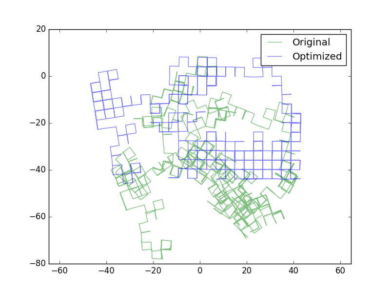
You may access my code here. It takes as input the pose-graph (in green). It optimizes a least squares cost function and produces the optimized poses (in blue). To understand the details of the cost function and how to solve the minimization problem (non-linear least squares) read on. You should be able to recreate the result here following the readme file on git of this project.

Pose Graph Optimization

Dataset

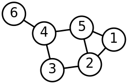
We represent pose at each time instant with a graph node. These poses can be obtained with odometry. But to concentrate just on the pose graph optimization aspect, we shall use the BAL Manhattan Dataset. This test dataset represents a graph with 3500 nodes and 5453 edges.  Pose are 3-DOF, ie motion in planar space (X,Y, theta)

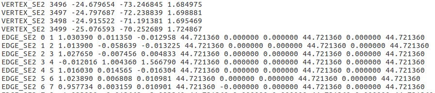
The dataset represents a bunch of vertices (VERTEX_SE2) represented as ID X Y Theta. These are unoptimized poses of each node represented in the world co-ordinate system. Each line starting with EDGE_SE2represents a relative pose between 2 nodes. This format is referred to as g2o format (not to be confused with g2o library) . For more details on this file refer to the Manhattan datasets website A snapshot of the dataset is as follows :

This text file is quite straight forward to read for example with C++ or Python. In this demo I shall use C++ as I wish to use Ceres-solver a popular library to solve large sparse optimization problem. Yet another popular libraries to solve pose graph optimization is g2o. I prefer to use Ceres-solver. In my gist look at ReadG2O::ReadG2O().

Least Squares Pose Graph Optimization – Theory

Basic Intuition

After beating around the bush, now its time to kill the tiger 😛 !!. We try and define the error terms at each edge. Final cost function is sum of squares of errors at each edge. We minimize this cost function with an iterative method say Gauss-Newton Method to tune the poses at each node. Note that here the poses at each node are the optimization variables and relative poses from edges are the observations.

If you do not understand the basics of non-linear least squares optimization, it will be worth while to complete a short tutorial on ceres-solver before continuing any further. Especially pay attention to exponential fitting example in ceres tutorial.

Notations

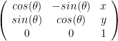
Consider an edge from node a to node b. Let be the planar pose on node a in world co-ordinate system. Similarly be the pose of node b in world co-ordinate system. Note that given x,y, theta (VERTEX_SE2) it is straight forward to comeup with matrices  and . Recall that a planar pose (ie. matrix group SE(2)) transformation matrix looks like:

We represent the edge observation (obtained from file.g2o - EDGE_SE2) with . It is important to distinguish between and . 

Cost Function

We argue that will give pose of node b in co-ordinate system of node a.  The difference pose shall be . Note that . Thus, the residue theta (del_theta=acos(D(0,0)) and residue displacement (del_x=D(0,2)) and (del_y=D(1,2) can be inferred from this matrix. This is literally it, almost all of the pose graph methods revolve around this concept.

More Resources

A good reference ppt can be found here. To get a more rigorous understanding, I would highly recommend you to read paper[3]. If you prefer a video lecture, I can highly recommend, SLAM course by Cyrill Stachniss. If you do not have enough time to view all the lecture, you may skip straight to lecture 15 of this series, which explains least squares pose-graph optimization, which is most relevant to this blog post.

Ceres Implementation Notes

Ceres-solver is an extremely flexible frame-work which basically solves a non-linear least squares optimization problem, specifically,

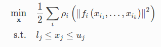
One need only supply the defination of the functions . It has automatic derivative computation to solve this optimization problem with variants of Gauss-Newton Methods. This function defination is exactly same as above 3 sub-sections. In my demo-code class PoseResidue defines the cost function for every edge. The function (in main) AddResidueBlock() sums the residue for every edge. 

Results

Robust Pose Graph Optimization

Very often the front end (data association/loop closure) modules produce outliers. In other words the loop closure modules produce false positives on account of self similar environment, perceptual aliasing etc. The naive approach to LS-SLAM fails catastrophically even in the presence of small number of false constraints.

I have put up a PPT on recent advances in robust pose graph optimization in presence of false loop closures. You may access the PPT here. I have implemented some of these advanced techniques with toy-examples. The whole repo can be found here: https://github.com/mpkuse/advanced_techniques_for_curvefitting/

References

[1] http://frc.ri.cmu.edu/~kaess/vslam_cvpr14/

[2] Bundler – Bundler: Structure from Motion (SfM) for Unordered Image Collections

[3] Grisetti, Giorgio, et al. “A tutorial on graph-based SLAM.” IEEE Intelligent Transportation Systems Magazine 2.4 (2010): 31-43.

[4] Cytill Stachniss’s Youtube SLAM Course

[5] Ceres-Solver Tutorial

Robust Pose Graph Optimization References

[1] Sünderhauf, Niko, and Peter Protzel. “Switchable constraints for robust pose graph SLAM.” Intelligent Robots and Systems (IROS), 2012 IEEE/RSJ International Conference on. IEEE, 2012.

[2] Olson, Edwin, and Pratik Agarwal. “Inference on networks of mixtures for robust robot mapping.” The International Journal of Robotics Research 32.7 (2013): 826-840.

[3] Pratik Agarwal, Gian Diego Tipaldi, Luciano Spinello, Cyrill Stachniss and Wolfram Burgard Robust Map Optimization using Dynamic Covariance Scaling Proceedings of the International Conference on Robots and Automation (ICRA), Karlsruhe, Germany, 2013