This terms quite often in computer vision related research papers. I am going to toyify it (a core simple explanation). All the code snippets are to be found along with the post. This is roughly a summarization of an excellent youtube-mini-series by Victor Lavrenko. The code snippets are my works.
Preliminaries
To understand this, you need to understand:
– Difference between datapoints and distribution (histogram of data points)
– The Gaussian function
– Bayes Rule
Datapoints and Distributions (Histogram)

Above we plot the histogram of the data. Please take a minute to review how that plot was made and what it means. It means that the datapoint ‘1’ occurs 2 times; the data point ‘2’ occurs 1 time; the datapoint ‘3’ occurs 2 times; the datapoint ‘4’ occurs 3 times; the datapoint ‘5’ occurs 1 time. When we say data distribution, we mean the histogram of the data. Lot of people get confused with this, so please be mindful. When we mean that the data distribution looks like a gaussian distribution it means that the histogram of the data’s graph closely resembles the gaussian-distribution equation.
The Gaussian Function
The equation 

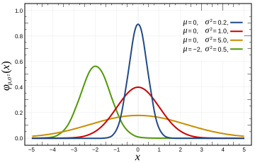
The function (the Gaussian) is often used as an approximation to represent the histogram. In other words, if someone says the data is gaussian distributed it means that if you plot the histogram of the data, then the histogram can be represented by the scary looking equation of this section.
One more point to know about Gaussian distribution is that when you evaluate the gaussian function at a particular x say 
Some other commonly used data distributions include: Uniform, Lognormal, Exponential, Boltzmann distribution etc. The wiki page on list of data distribution functions is a good exploratory resource. It is important to understand that these standard data distributions merely provide a analytical tool to model data. The underlying data may not follow those distributions.
Since our data was 1D a simple histogram could suffice, however for higher dimensional data the histogram would be a surface plot like below. For higher dimensional data we cannot imagine the distribution with such a plot.

Bayes Rule
The Bayes rule is one of the corner stones of probability analysis. The crux of it come in 2 (or more) events occurring together. Imagine 2 events something like a) it will rain b) I will be sick. And say we are interested in analyzing the probability that it will rain AND I will be sick (


The Bayes rule is derived from these two statements above:

The prime usage of it is when you have conditional probability and you want to invert the conditions (P(A/B) and P(B/A) are said to be inverse of each other).
Gaussian Mixture Models
Imagine you have some 1D datapoints (in blue, in plot below). And say we are tasked with representing this data in an analytical form. We could represent the underlying data by a single gaussian but it won’t be accurate enough. So the idea is to use multiple gaussians to represent a distribution. In this case we know from visual inspection that 3 gaussians can represent this data with sufficient accuracy. Now our task is to know what are these 3 gaussians. Note that a gaussian is fully defined by its mean and variance (

One Gaussian Fitting
Before we attempt to know about 3 gaussians, lets deal with 1 gaussian case. The task is given n data points, find a gaussian distribution that fits it.
# Given Input Data
x = [ 19.94052346   6.30157208  12.08737984  24.70893199  20.9755799
  -7.4727788   11.80088418   0.78642792   1.26781148   6.40598502
   3.74043571  16.84273507   9.91037725   3.51675016   6.73863233
   5.63674327  17.24079073   0.24841736   5.43067702  -6.24095739]


# Task: Fit a Gaussian on this data
sample_mu = np.mean( x )
sample_sigma = np.sqrt( np.var( x ) )
print 'sample_mu=', sample_mu, '\tsample_sigma=', sample_sigma
#     ^^^ prints: sample_mu= 7.99334592946 	sample_sigma= 8.50182800399

# Plot histogram and overlay it with Gaussian plot
def gauss( t, mu, sigma ):
    return 1.0 / np.sqrt( 2*np.pi * sigma**2 ) * np.exp( -(t - mu)**2 / (2*sigma**2) )

probabilities, datapts  = np.histogram( x,normed=True  )

plt.plot( datapts[0:-1], probabilities, 'r-.' )
t = np.linspace( -50, 50, 100 )
plt.plot( t, gauss( t, sample_mu, sample_sigma), 'b-' )
plt.plot( x, .01 + np.zeros( len(x)), 'g*' )
plt.show()

Multiple Gaussian Fitting
Before reading this section, I highly recommend you watch the videos (20min) by Victor Lavenko.
So, if we are given the data points and we know which of the K gaussians a particular datapoint belongs, we could find the means and variances of those gaussians. On the other hand if we know the means and variances of each of those K gaussians we could associate each of the datapoints to the gaussians. We can do this by computing the probability that this point belongs to each of the K gaussians. We can assign the datapoint to the gaussian with maximum probability.
This is like a chicken-and-egg problem. But in a real case we neither know the data associations with the gaussians, nor do we know the means and variances of the gaussians.
To get around this issue, we could start with some initial guesses of means and variances. Using these we can figure out the data associations of each of the data points. Finally we could update the means and variance based on this new association. We could repeat this process. This is the crux of the EM algorithm for fitting a mixture of gaussian. Here is how it can be done with python script. Follow the code carefully and the comments to know how to implement it.
## Generate Data
observed_data = generate_1d_data()

## Initial Guess
K = 2
est_mu = np.ones(K)
est_sigma = np.ones(K)

est_mu[0] = 0.0
est_sigma[0] = 8.
est_mu[1] = 8.0
est_sigma[1] = 8.


## Simplistic
# loopover all data points
P_classj_given_x = np.ones( (len(observed_data), K) )
for i in range( len(observed_data) ):
    x = observed_data[i]
    p_x_given_a = gauss( x,  est_mu[0], est_sigma[0] ) #what is the probability that it belongs to class-A
    p_x_given_b = gauss( x,  est_mu[1], est_sigma[1] ) #what is the probability that it belongs to class-B

    # Using bayes law ,
    #   p_classj_given_xi := p_x_given_classj \times p_b / ( \sum_k p_x_given_class_k \times p_class_k )
    p_a = 0.5 #prior probability
    p_b = 0.5
    p_class_a_given_xi = ( p_x_given_a * p_a ) / (  p_x_given_a * p_a  +  p_x_given_b * p_b  )
    p_class_b_given_xi = ( p_x_given_b * p_b ) / (  p_x_given_a * p_a  +  p_x_given_b * p_b  )

    print 'i=%3d)   x_%d=%4.2f\tp_x_given_a=%4.4f\tp_x_given_b=%4.4f  <==>  p_class_a_given_xi=%4.4f\tp_class_b_given_xi=%4.4f' %( i, i, x, p_x_given_a, p_x_given_b,    p_class_a_given_xi, p_class_b_given_xi )
    P_classj_given_x[ i, 0 ] = p_class_a_given_xi
    P_classj_given_x[ i, 1 ] = p_class_b_given_xi


# comute new estimates based on `p_class_a_given_xi` and `p_class_a_given_xi`
mu0_next = np.dot( P_classj_given_x[:,0] , observed_data ) / np.sum(P_classj_given_x[:,0])
sigma0_next = np.sqrt(   np.dot(   P_classj_given_x[:,0], (observed_data - mu0_next)**2   )  / np.sum(P_classj_given_x[:,0]) )
#

mu1_next = np.dot( P_classj_given_x[:,1] , observed_data ) / np.sum(P_classj_given_x[:,1])
sigma0_next = np.sqrt(   np.dot(   P_classj_given_x[:,0], (observed_data - mu0_next)**2   )  / np.sum(P_classj_given_x[:,0]) )

print 'mu0_next=', mu0_next, '\tsigma0_next=', sigma0_next
print '\n', 'mu1_next=', mu1_next

Multiple Gaussian Fitting : Iterative Estimation
The above was only one iteration, we could repeat the above process to refine the estimate further. I am showing the output here, I have implemented it in my repo : https://github.com/mpkuse/gmm_pointcloud_align. Do check out the code to know the details.
====GMMFit::fit_1d====
Initial Guess:
#0	mu=0	sigma=5
#1	mu=10	sigma=5
initial priors: 0.5 0.5
---itr=0
Likelihood Computation
Posterior Computation (Bayes Rule)
Update mu, sigma
mu_new_0 1.28913	sigma_new_0 5.60456
mu_new_1 14.6433	sigma_new_1 6.80517
Update priors
updated priors: 0.276415 0.723585
---itr=1
Likelihood Computation
Posterior Computation (Bayes Rule)
Update mu, sigma
mu_new_0 1.62944	sigma_new_0 5.77318
mu_new_1 14.5001	sigma_new_1 7.01016
Update priors
updated priors: 0.275672 0.724328
---itr=2
Likelihood Computation
Posterior Computation (Bayes Rule)
Update mu, sigma
mu_new_0 1.85894	sigma_new_0 5.93708
mu_new_1 14.3973	sigma_new_1 7.12795
Update priors
updated priors: 0.274779 0.725221
---itr=3
Likelihood Computation
Posterior Computation (Bayes Rule)
Update mu, sigma
mu_new_0 2.03784	sigma_new_0 6.0696
mu_new_1 14.3194	sigma_new_1 7.21106
Update priors
updated priors: 0.274183 0.725817
---itr=4
Likelihood Computation
Posterior Computation (Bayes Rule)
Update mu, sigma
mu_new_0 2.18404	sigma_new_0 6.17629
mu_new_1 14.2582	sigma_new_1 7.27433
Update priors
updated priors: 0.273825 0.726175
---itr=5
Likelihood Computation
Posterior Computation (Bayes Rule)
Update mu, sigma
mu_new_0 2.30649	sigma_new_0 6.2636
mu_new_1 14.2089	sigma_new_1 7.32442
Update priors
updated priors: 0.273633 0.726367
---itr=6
Likelihood Computation
Posterior Computation (Bayes Rule)
Update mu, sigma
mu_new_0 2.41079	sigma_new_0 6.33631
mu_new_1 14.1685	sigma_new_1 7.36507
Update priors
updated priors: 0.27356 0.72644
---itr=7
Likelihood Computation
Posterior Computation (Bayes Rule)
Update mu, sigma
mu_new_0 2.50078	sigma_new_0 6.39776
mu_new_1 14.1347	sigma_new_1 7.39868
Update priors
updated priors: 0.273571 0.726429
---itr=8
Likelihood Computation
Posterior Computation (Bayes Rule)
Update mu, sigma
mu_new_0 2.57925	sigma_new_0 6.45035
mu_new_1 14.1064	sigma_new_1 7.42685
Update priors
updated priors: 0.273646 0.726354
---itr=9
Likelihood Computation
Posterior Computation (Bayes Rule)
Update mu, sigma
mu_new_0 2.64828	sigma_new_0 6.49582
mu_new_1 14.0823	sigma_new_1 7.45074
Update priors
updated priors: 0.273769 0.726231
==== DONE GMMFit::fit_1d====

